 This is the fifth post in an article series about MIT's Linear Algebra course. In this post I will review lecture five that finally introduces real linear algebra topics such as vector spaces their subspaces and spaces from matrices. But before it does that it closes the topics that were started in the previous lecture on permutations, transposes and symmetric matrices.
Here is a list of the previous posts in this article series:
- Lecture 1: Geometry of Linear Equations
- Lecture 2: Elimination with Matrices
- Lecture 3: Matrix Multiplication and Inverse Matrices
- Lecture 4: A=LU Factorization
Lecture 5: Vector Spaces and Subspaces
Lecture starts with reminding some facts about permutation matrices. Remember from the previous lecture that permutation matrices P execute row exchanges and they are identity matrices with reordered rows.
Let's count how many permutation matrices are there for an nxn matrix.
For a matrix of size 1x1, there is just one permutation matrix - the identity matrix.
For a matrix of size 2x2 there are two permutation matrices - the identity matrix and the identity matrix with rows exchanged.
For a matrix of size 3x3 we may have the rows of the identity matrix rearranged in 6 ways - {1,2,3}, {1,3,2}, {2,1,3}, {2,3,1}, {3,1,2}, {3,2,1}.
For a matrix of size 4x4 the number of ways to reorder the rows is the same as the number of ways to rearrange numbers {1,2,3,4}. This is the simplest possible combinatorics problem. The answer is 4! = 24 ways.
In general, for an nxn matrix, there are n! permutation matrices.
Another key fact to remember about permutation matrices is that their inverse P-1 is their transpose PT. Or algebraically PT·P = I.
The lecture proceeds to transpose matrices. The transpose of a matrix exchanges its columns with rows. Another way to think about it that it flips the matrix over its main diagonal. Transpose of matrix A is denoted by AT.
Here is an example of transpose of a 3-by-3 matrix. I color coded the columns to better see how they get exchanged:

A matrix does not have to be square for its transpose to exist. Here is another example of transpose of a 3-by-2 matrix:

In algebraic notation transpose is expressed as (AT)ij = Aji, which says that an element aij at position ij get transposed into the position ji.
Here are the rules for matrix transposition:
- The transpose of A + B is (A + B)T = AT + BT.
- The transpose of A·B is (A·B)T = BT·AT.
- The transpose of A·B·C is (A·B·C)T = CT·BT·AT.
- The transpose of A-1 is (A-1)T = (AT)-1.
Next the lecture continues with symmetric matrices. A symmetric matrix has its transpose equal to itself, i.e., AT = A. It means that we can flip the matrix along the diagonal (transpose it) but it won't change.
Here is an example of a symmetric matrix. Notice that the elements on opposite sides of the diagonal are equal:

Now check this out. If you have a matrix R that is not symmetric and you multiply it with its transpose RT as R·RT, you get a symmetric matrix! Here is an example:

Are you wondering why it's true? The proof is really simple. Remember that matrix is symmetric if its transpose is equal to itself. Now what's the transpose of the product R·RT? It's (R·RT)T = (RT)T·RT = R·RT - it's the same product, which means that R·RT is always symmetric.
Here is another cool fact - the inverse of a symmetric matrix (if it exists) is also symmetric. Here is the proof. Suppose A is symmetric, then the transpose of A-1 is (A-1)T = (AT)-1. But AT = A, therefore (AT)-1 = A-1.
At this point lecture finally reaches the fundamental topic of linear algebra - vector spaces. As usual, it introduces the topic by examples.
Example 1: Vector space R2 - all 2-dimensional vectors. Some of the vectors in this space are (3, 2), (0, 0), (?, e) and infinitely many others. These are all the vectors with two components and they represent the xy plane.
Example 2: Vector space R3 - all vectors with 3 components (all 3-dimensional vectors).
Example 3: Vector space Rn - all vectors with n components (all n-dimensional vectors).
What makes these vectors vector spaces is that they are closed under multiplication by a scalar and addition, i.e., vector space must be closed under linear combination of vectors. What I mean by that is if you take two vectors and add them together or multiply them by a scalar they are still in the same space.
For example, take a vector (1,2,3) in R3. If we multiply it by any number ?, it's still in R3 because ?·(1,2,3) = (?, 2?, 3?). Similarly, if we take any two vectors (a, b, c) and (d, e, f) and add them together, the result is (a+d, b+e, f+c) and it's still in R3.
There are actually 8 axioms that the vectors must satisfy for them to make a space, but they are not listed in this lecture.
Here is an example of not-a-vector-space. It's 1/4 of R2 (the 1st quadrant). The green vectors are in the 1st quadrant but the red one is not:
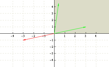 An example of not-a-vector-space.
This is not a vector space because the green vectors in the space are not closed under multiplication by a scalar. If we take the vector (3,1) and multiply it by -1 we get the red vector (-3, -1) but it's not in the 1st quadrant, therefore it's not a vector space.
Next, Gilbert Strang introduces subspaces of vector spaces.
For example, any line in R2 that goes through the origin (0, 0) is a subspace of R2. Why? Because if we take any vector on the line and multiply it by a scalar, it's still on the line. And if we take any two vectors on the line and add them together, they are also still on the line. The requirement for a subspace is that the vectors in it do not go outside when added together or multiplied by a number.
Here is a visualization. The blue line is a subspace of R2 because the red vectors on it can't go outside of line:
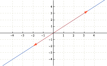 An example of subspace of R2.
And example of not-a-subspace of R2 is any line that does not go through the origin. If we take any vector on the line and multiply it by 0, we get the zero vector, but it's not on the line. Also if we take two vectors and add them together, they are not on the line. Here is a visualization:
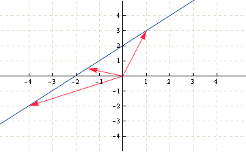 An example of not-a-subspace of R2.
Why not list all the subspaces of R2. They are:
- the R2 itself,
- any line through the origin (0, 0),
- the zero vector (0, 0).
And all the subspaces of R3 are:
- the R3 itself,
- any line through the origin (0, 0, 0),
- any plane through the origin (0, 0, 0),
- the zero vector.
The last 10 minutes of the lecture are spent on column spaces of matrices.
The column space of a matrix is made out of all the linear combinations of its columns. For example, given this matrix:

The column space C(A) is the set of all vectors {?·(1,2,4) + ?·(3,3,1)}. In fact, this column space is a subspace of R3 and it forms a plane through the origin.
More about column spaces in the next lecture.
You're welcome to watch the video lecture five:
Topics covered in lecture five:
- [01:30] Permutations.
- [03:00] A=LU elimination without row exchanges.
- [03:50] How Matlab does A=LU elimination.
- [04:50] PA=LU elimination with row exchanges
- [06:40] Permutation matrices.
- [07:25] How many permutation matrices are there?
- [08:30] Permutation matrix properties.
- [10:30] Transpose matrices.
- [11:50] General formula for transposes: (AT)ij = Aji.
- [13:06] Symmetric matrices.
- [13:30] Example of a symmetric matrix.
- [15:15] R·RT is always symmetric.
- [18:23] Why is R·RT symmetric?
- [20:50] Vector spaces.
- [22:05] Examples of vector spaces.
- [22:55] Real vector space R2.
- [23:20] Picture of R2 - xy plane.
- [26:50] Vector space R3.
- [28:00] Vector space Rn.
- [30:00] Example of not a vector space.
- [32:00] Subspaces of vector spaces.
- [33:00] A vector space inside R2.
- [34:35] A line in R2 that is subspace.
- [34:50] A line in R2 that is not a subspace.
- [36:30] All subspaces of R2.
- [39:30] All subspaces of R3.
- [40:20] Subspaces of matrices.
- [41:00] Column spaces of matrices C(A).
- [44:10] Example of column space of matrix with columns in R3.
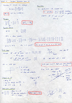
Here are my notes of lecture five:
The next post is going to be more about column spaces and null spaces of matrices.

